Complexity Analysis¶

Computational complexity analysis plays a pivotal role in the theoretical analysis of algorithms. It involves assessing how the performance of an algorithm scales with the size of the input, enabling us to make predictions about an algorithm’s efficiency in terms of time and space usage. This analysis is crucial for understanding the inherent difficulty of solving computational problems and for comparing and selecting algorithms for various tasks.

Concepts¶

Computational complexity¶: The computational resources consumed by an algorithm as a function of the size of the problem.
Time complexity¶: The computational time consumed by an algorithm as a function of the size of the problem. It is usually described using a function \(T(n)\).
Space complexity¶: The computational storage space (usually refer to memory) consumed by an algorithm as a function of the size of the problem. auxiliary space complexity is the space complexity excluding the input data. It is usually described using a function \(S(n)\).
Best case, worst case, and average case¶: Best case is the scenario in which the algorithm finished with the least resource consumed. Worst case is the scenario in which the algorithm finished with the most resource consumed. Sometimes we will use average case, which is the average over all possible inputs.
Constant time operation¶: Because the accurate measurement of time consumption is impossible, we usually count the number of constant time operations to estimate the time consumption. A constant time operation is an operation that always consume a certain amount of time regardless of the problem size n.
Growth rate¶: How much more resource is needed when the problem size grows. It is usually described using simple math functions. It is a simple way to visualize the complexity.

Asymptotic notation¶

Asymptotic notation is the math language we use to describe the complexity in a formal way. It is formally known as Bachmann–Landau notation. A mathematical notation system to describe the limiting behavior of a function. It includes \(O\) (big-O), \(\Omega\) (big-omega), \(\Theta\) (big-theta) notations.

Note

Time complexity is more useful and is focused in the following sections. Most of the rules can be used with space complexity with little modification.

Motivation¶

Time, space or other kind of complexities are functions of the problem size \(n\). They are not too helpful to describe the complexity of an algorithm for the following reason:

They can be very complex functions that cannot be easily described or compared.
They can be very different for different problem sizes, while we are more interested in the general trend when the problem size grows large.

Thus, we need a method to describe the complexity as simpler math functions and focus on the general trend when the problem size grows large.

E.g. \(T(n) = 3n^2 + 10n + 4\) is a time function of a certain algorithm. It can be simplified to asymptotic notation \(\Theta(n^2)\), which is good enough to describe how the resource consumption grows with the problem size when the problem size is large.

Formal Definitions¶

Given \(T(n)\) the time function of the problem size \(n\)

We will write \(T(n) = O(f(n))\) or \(T(n) \in O(f(n))\) if there exists a certain positive constant \(c\) and a problem size \(n_{0}\), such that \(T(n) \leq cf(n)\) for all \(n \geq n_{0}\).

We will write \(T(n) = \Omega(f(n))\) or \(T(n) \in \Omega(f(n))\) if there exists a certain positive constant \(c\) and a problem size \(n_{0}\), such that \(T(n) \geq cf(n)\) for all \(n \geq n_{0}\).

We will write \(T(n) = \Theta(f(n))\) if \(T(n) = \Omega(f(n))\) and \(T(n) = O(f(n))\) are both true. Note: the constants are different.

We will write \(T(n) = o(f(n))\) or \(T(n) \in O(f(n))\) if there exists a certain positive constant \(c\) and a problem size \(n_{0}\), such that \(T(n) < cf(n)\) for all \(n \geq n_{0}\).

Warning

The \(=\) used in equations like \(T(n) = O(f(n))\) does not mean equal! It means in or belong to.

All notations \(O(f(n))\), \(\Omega(f(n))\), and \(\Theta(f(n))\) define sets of functions that have the same order. Thus, the set will be the same of the function \(f(n)\) has the same order. For example, \(\Theta(n^2)=\Theta(2*n^2)=\Theta(n^2+3n)=\dots\) so we can use the simplest form of the function to represent the set.

How they work and which one to choose¶

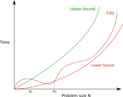
For a complexity, there exist infinite upper and lower bounds and we should focus on the “tightest” bound.
If a big theta notation exists, it is guaranteed to be the tightest upper and lower bound.
The big theta notation, \(\Theta(f(n))\) is the most precise notation and is preferred as possible. However, it may not always exist in practice.
When we cannot find the big theta notation, we can use big O \(O(f(n))\) to describe the upper bound of the complexity. As it describe the upper bound, which is a guarantee that the complexity will not exceed this value.

E.g. \(T(n) = 3n^2 + 10n + 4\) is a time function of a certain algorithm. It has the big theta notation \(\Theta(n^2)\), which is the tightest bound. It also has the tightest upper bound \(O(n^2)\) and tightest lower bound \(\Omega(n^2)\). Other upper bounds like \(O(n^3)\), \(O(n^4)\) are also valid but not as tight as \(O(n^2)\). Other lower bounds like \(\Omega(n)\), \(\Omega(\log n)\) are also valid but not as tight as \(\Omega(n^2)\).

E.g. Mark Zuckerberg’s income is an upper bound to your income but it is not helpful to estimate your income because it is not a “tight” upper bound.

Considering Cases¶

In complexity analysis, various cases are considered to assess the efficiency and performance of algorithms. These cases help us understand how algorithms behave under different scenarios and input distributions.

Best Case: The minimum amount of resources required by the algorithm.
Worst Case: The maximum amount of resources required by the algorithm.
Average Case: The average amount of resources required by the algorithm.

Warning

Bounds and cases are not directly related. Do not treat upper bound as worst case and lower bound as best case!

Each case provides a complexity as a function of problem size and we can use upper/lower/exact bound to estimate the growth rate of this function.

Representative Algorithms of Certain Complexity¶

Typical Complexity and Representative Algorithms¶
Name	Bound (prefer big theta)	Representative Algorithms
Constant	\(\Theta(1)\)	Array indexing, Hash table lookups
Logarithmic	\(\Theta(\log n)\)	Binary Search, Balanced Binary Search Trees (e.g., AVL, Red-Black)
Linear	\(\Theta(n)\)	Linear Search, Most Simple Array/Linked List Operations
Linearithmic	\(\Theta(n \log n)\)	Merge Sort, Heap Sort, Quick sort
Quadratic	\(\Theta(n^2)\)	Bubble Sort, Selection Sort, Insertion Sort
Polynomial (k > 2)	\(\Theta(n^k)\)	Matrix Multiplication (naive approach)
Exponential	\(\Theta(2^n)\)	Recursive algorithms without memoization (e.g., naive Fibonacci)
Factorial	\(\Theta(n!)\)	Traveling Salesman Problem (naive solution)

Properties¶

\(\Theta(f(n))\) is a set of functions that have the same order as \(f(n)\).
- E.g. \(\Theta(n^2) = \Theta(2n^2) = \Theta(n^2 + 3n) = \dots\) because they all have the same order \(n^2\).
- Thus, we will always use the simplest form of \(f(n)\) to represent the set. E.g. \(\Theta(2n^2 + 10n - 4) = \Theta(n^2)\). This step is called simplification.
If \(T(n) = \Theta(f(n))\) and \(g(n)\) is a function with higher order than \(f(n)\), then \(T(n) = \Theta(g(n))\).
- E.g. if \(T(n) = 3n^2 + 10n + 4 = \Theta(n^2)\), then \(T(n) = \Theta(n^3) = \Theta(n^4) = \cdots\), All functions with higher order than \(n^2\) is a possible upper bound of \(T(n)\).
- Thus, we should always use the lowest-possible order to represent the set, \(\Theta(n^2)\) in this case. Because higher order functions is always a possible upper bound, they become less meaningful.
Summary, We should always use the simplest form of the lowest-possible order to represent the set.

Steps to Find Complexity¶

Option 1: Find \(T(n)\) and then find \(\Theta(f(n))\).
Option 2: Estimate \(\Theta(f(n))\) directly.

Find \(T(n)\)¶

\(T(n)\) = number of operations
Count the number of constant time operations
Each statement, and expression evaluation is considered to take constant time.
- E.g. In the pseudo code if a < 10 then b = a + 10, the comparison a < 10 and the assignment b = a + 10 are considered to take constant time. They both should be counted as 1 operation.
Function calls are more complicated. Functions that does not variable size input are mostly constant time. Functions that does variable size input are more complicate and you better check the reference.
- std::swap, cout <<, getline are constant time.
- std::sort, std::search, std::shuffle are not constant time.

Find \(\Theta\) given \(T(n)\)¶

Keep the term with highest order. Drop the coefficient and lower order terms go provide the simplest form.
Example:
- \(T(n) = 20 \times n^2 + 10 \times n + 12 = \Theta(n^2)\)
- \(T(n) = 5 \times 2^n + 3 \times n^3 = \Theta(2^n)\)

Common Growth Rates, from low to high order¶
Term	Growth Rate
Constant Time	\(1\)
Logarithmic	\(\log n\)
Linear	\(n\)
Linearithmic	\(n \log n\)
Quadratic	\(n^2\)
Cubic	\(n^3\)
Exponential	\(2^n\)
Factorial	\(n!\)

Find \(\Theta\) directly¶

additive (sequential, branch)
- \(\Theta(f(n)) + \Theta(g(n)) = \Theta(f(n) + g(n))\)
- E.g. \(\Theta(n^2) + \Theta(n) = \Theta(n^2 + n) = \Theta(n^2)\)
multiplicative (loop, recursion)
- for a layer of loop: \(\Theta(f(n)) \times \Theta(g(n)) = \Theta(f(n) \times g(n))\)
- complexity of number of iterations \(\Theta(f(n))\)
  - how problem size is reduced in each iteration`
  - reduce by half each round: \(\Theta(\log n)\)
  - reduce by a constant each round: \(\Theta(n)\)
- complexity in each iteration \(\Theta(g(n))\)
- E.g. For merge sort, the number of iterations is \(\Theta(\log n)\) and the complexity in each iteration is \(\Theta(n)\). Thus, the total complexity is \(\Theta(\log n) \times \Theta(n) = \Theta(n \log n)\).

Pitfalls¶

Confusing \(T(n)\) to \(\Theta(f(n))\)
Not all function calls are constant time operations (a.k.a. \(\Theta(1)\))