Data Structure and Algorithm Design II
Chapter 11
Xingang (Ian) Fang
Sections
Graph
Graph Traversal Algorithms
Topological Sort Algorithm
Minimum Spanning Tree Algorithms
Shortest Path Algorithms
Graph
Xingang (Ian) Fang
Outline
Overview
Concepts
Example graphs
Representations
Algorithms
Overview
Graphs are a fundamental data structure in computer science.
Graphs are used to model networks, complex relationships, etc.
Vertices(nodes) connected by edges.
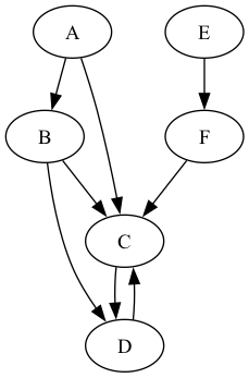
Applications
Social networks
Routing algorithms
Computer networks
Transportation and logistics
Machine learning/deep learning
Bioinformatics
Integrated circuit design
Database systems
Computer vision
Optimization problems
Game development
Concepts
Vertex/Node
degree of vertex: number of neighbors
Edge/Arc
directed/undirected
weighted/unweighted
Connectivity
path between two vertices
length of path
distance between two vertices
adjacent
connected / unconnected
cyclic / acyclic
Graph level properties
degree of graph: max degree of vertices
directed/undirected
weighted/unweighted
cyclic/acyclic
connected/unconnected
dense/sparse
Graph Examples
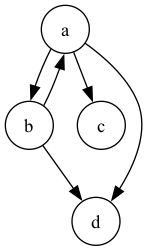
Directed connected cyclic graph
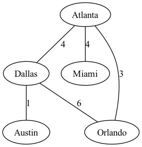
Undirected connected cyclic weighted graph
Graph Examples (contd.)
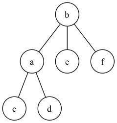
Undirected connected acyclic graph (Tree)
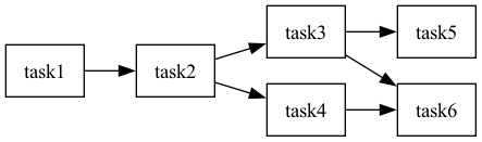
Directed acyclic graph (DAG) task planning
Representations
Compare adjacency matrices and lists in our Graph Representation Lab.
Vertices with pointers to neighbors (uncommon)
List of edges
A list of edges is a 1d array in which every element in the array represents an edge. It is the simplest way to represent a graph. It is also an easy way to store a graph in a relational database. It is not efficient for most graph algorithms though.
Adjacency list
An adjacency list is a 1d array in which every element in the array represents a vertex and points to a list of its neighbors.
Adjacency matrix
An adjacency matrix is a 2d array in which each row represents a source vertex and each column represents a destination vertex. The elements in the matrix represents the edge between the two vertices.
Algorithms
Graph traversal
Breadth-first search
Depth-first search
Step through both in our BFS & DFS Graph Explorer.
Topological sort (DAG only)
Shortest path
Dijkstra’s algorithm (single source, greedy)
Floyd-Warshall Algorithm (all pairs, dynamic programming)
Minimum spanning tree
Prim’s algorithm (greedy)
Kruskal’s algorithm (greedy)
Graph Traversal
Overview
Depth First Search (DFS)
Breadth First Search (BFS)
Visualization
Overview
Start from a vertex
Visit all reachable vertices connected to it in a systematic order
Two common ways to traverse a graph
Depth First Search (DFS)
Breadth First Search (BFS)
Depth First Search (DFS)
Like walking in a maze, you go as far as you can, then backtrack
Stack based implementation
function dfs(startVertex):
  create a new stack

  push startVertex onto the stack
  mark startVertex as visited

  while the stack is not empty:
    current = pop from the stack
    process(current)  # Perform an action on the current node

    for each neighbor in current.neighbors:
      if neighbor is not in visited set:
        push neighbor onto the stack
        add neighbor to the visited set
Recursive implementation
function dfs(vertex, visited):
  if vertex is not visited:
    mark vertex as visited
    visit(node)  # Perform an action on the vertex

    for each neighbor of the vertex:
      if neighbor is not visited:
          dfs(neighbor, visited)
Breadth First Search (BFS)
Like a wave, you visit all vertices at the same level before going deeper
Queue based implementation
function bfs(startVertex):
  create a new queue

  enqueue the startVertex
  mark the startVertex as visited

  while the queue is not empty:
    dequeue a vertex from the queue
    process(vertex)  # Perform an action on the vertex

    for each neighbor of the vertex:
      if neighbor is not visited:
        mark the neighbor as visited
        enqueue the neighbor
Visualization
Topological sort
Overview
Algorithm
Overview
Only works on directed acyclic graphs (DAGs)
Will provide a unique ordering of the vertices if the order of of vertices in the graph is unique
Will provide a linear ordering of the vertices
Applications and Use cases
Task scheduling
Dependency resolution
Compiler optimization
Algorithm
For every vertex, use DFS to find all vertices reachable from it
Add the vertex to a result list after the recursive call
Reverse the result list to get the topological sort
Our BFS & DFS Graph Explorer steps through the DFS traversal used by topological sort.
function topologicalSort(graph):
  initialize an empty list 'result' to store the topological order
  initialize a set 'visited' to keep track of visited nodes

  for each node 'v' in graph:
    if 'v' is not in 'visited':
      performDFS(v, visited, result)

return 'result' in reverse order

function performDFS(node, visited, result):
  mark 'node' as visited
  for each neighbor 'n' of 'node':
    if 'n' is not in 'visited':
      performDFS(n, visited, result)
  append 'node' to 'result'
Minimum Spanning Tree
Overview
Prim’s Algorithm
Kruskal’s Algorithm
Comparison
Visualization
Overview
A spanning tree of a graph is a subgraph that contains all the vertices of the graph and is a tree.
A minimum spanning tree (MST) of a weighted graph is a spanning tree whose total weight is minimum.
Prim’s Algorithm
Kruskal’s Algorithm
Other
Boruvka’s Algorithm
Reverse-Delete Algorithm
Prim’s Algorithm
Greedy
Vertex based
Use a priority queue
Steps
Create an empty MST.
Initialize a priority queue with all vertices and their respective weights.
Start with an arbitrary vertex as the current vertex.
Mark the current vertex as visited.
While the priority queue is not empty:
Dequeue the vertex with the smallest weight from the priority queue.
If the dequeued vertex is not in the MST, add it to the MST and update its neighbors’ weights in the priority queue.
Repeat steps 4-5 until all vertices are in the MST.
Kruskal’s Algorithm
Greedy
Edge based
Use a disjoint set and a sorted edge list
Steps
Create an empty MST.
Sort all edges in the graph in ascending order of their weights.
Initialize a disjoint-set data structure to keep track of connected components.
For each edge in sorted order:
If adding the edge to the MST does not create a cycle, add it to the MST.
Repeat step 4 until the MST has (n-1) edges, where n is the number of vertices in the graph.
Comparison
Comparison Criteria |
Prim’s Algorithm |
Kruskal’s Algorithm |
Type |
Greedy |
Greedy |
Graph elements |
Vertices |
Edges |
Efficient for |
Dense graphs |
Sparse graphs |
Data structure/ADT |
Priority queue |
Disjoint-set |
Parallelization |
Not suitable |
Suitable |
Connected results |
Yes |
Yes (extra step) |
Visualization
Shortest Path Algorithms
Overview
Dijkstra’s Algorithm (Single Source Shortest Path)
Floyd-Warshall Algorithm (All Pairs Shortest Path)
Overview
Shortest Path Problem: Given a weighted graph G, find the shortest path
Single Source Shortest Path (SSSP): from a source vertex to all other vertices in G
All Pairs Shortest Path (APSP): among all pairs of vertices in G.
Algorithms
Dijkstra’s Algorithm (SSSP)
Floyd-Warshall Algorithm (APSP)
Applications
Network routing
GPS navigation
Optimization problems
Dijkstra’s Algorithm
Single source shortest path algorithm
Greedy algorithm
visualization
function dijkstra(graph, source):
  create a priority queue PQ
  initialize distances to all vertices as infinity
  set the distance to the source as 0
  enqueue source to PQ

  while PQ is not empty:
    current_vertex = vertex with the smallest distance in PQ
    remove current_vertex from PQ

    for each neighbor of current_vertex:
      edge_weight = weight of the edge between current_vertex and neighbor
      tentative_distance = distance to current_vertex + edge_weight
      if tentative_distance < distance to neighbor:
        set distance to neighbor as tentative_distance
        add neighbor to PQ
Floyd-Warshall Algorithm
All pairs shortest path algorithm
Dynamic programming
Visualization https://www.cs.usfca.edu/~galles/visualization/Floyd.html
function floyd_warshall(graph):
  initialize a distance matrix with infinite values
  set diagonal entries to 0 (distance to itself)

  for each edge (u, v) with weight w in the graph:
    set distance[u][v] = w

  for k in all vertices:
    for i in all vertices:
      for j in all vertices:
        if distance[i][j] > distance[i][k] + distance[k][j]:
          set distance[i][j] = distance[i][k] + distance[k][j]