Data Structure and Algorithm Design II
Module 4
Xingang (Ian) Fang
Sections
B tree and variants
Introduction to problem and algorithm classification
B-Tree and Variants
Xingang (Ian) Fang
Outline
Overview
Operations
Variants
Overview
Invented by Bayer and McCreight in 1972.
A M-ary search tree that stores data in order.
A balanced tree with all leaves at the same depth.
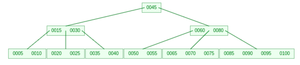
Definition: A B-tree of order \(m\) is a tree which satisfies the following properties:
Every node has at most \(m\) children.
Every internal node has at least \(\lceil m/2 \rceil\) children.
The root has at least 2 children if it is not a leaf node.
All leaves appear on the same level.
A non-leaf node with \(k\) children contains \(k-1\) keys.
Operations
Insertion
Start at the root node.
Find the leaf node where the key should be inserted.
If the node is not full, insert the key into the node.
If the node is full, split the node into two nodes.
Insert the median key into the parent node.
If the parent node is full, split the parent node.
Repeat until the root node is reached
Deletion
Start at the root node.
Find the node where the key should be deleted.
If the node is a leaf node, delete the key from the node.
If the node is an internal node, replace the key with the predecessor or successor key. Then delete the predecessor or successor key from the leaf node.
If the node is underfilled, borrow a key from a sibling node.
If the node is underfilled and no sibling node can lend a key, merge the node with a sibling node.
If the merge causes the parent node to be underfilled, repeat the process on the parent node.
Repeat until the root node is reached
Checkpoint
Why do all internal nodes have a lower bound of \(\lceil m/2 \rceil\) children?
Why does the room node have a lower bound of 2 children instead?
Is insertion always happening at the leaf node?
Is deletion always happening at the leaf node?
How are the implementation of the behaviors compared to that of a binary search tree?
Variants
2-3 Tree: A B-tree of order 3.
2-3-4 Tree: A B-tree of order 4.
B+ Tree: A B-tree of order \(m\) where all keys are stored in the leaves.
B* Tree: A B-tree of order \(m\) where all leaves are at least half full.
B# Tree: A B-tree of order \(m\) where all leaves are at least 2/3 full.
etc.
2-3 Tree
FYI
A B-tree of order 3.
Can be implemented as a binary search tree (red-black tree).
B+ Tree
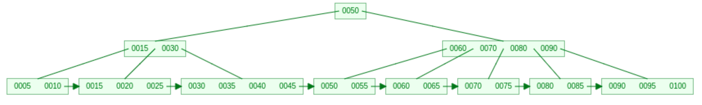
Definition: A B+ tree of order \(m\) satisfies the following properties:
All data are stored in the leaves.
All leaves are linked together.
All internal nodes are keys only for faster search.
All internal nodes have between \(\lceil m/2 \rceil\) and \(m\) children.
All leaves have between \(\lceil l/2 \rceil\) and \(l\) keys.
Works well with sequential access.
Ideal for file system and database indexing.
Reduced number of disk accesses.
Reduced redistribution of data when inserting or deleting.
Checkpoint
What is the difference between a B-tree and a B+ tree?
Why the sequential access is faster in a B+ tree?
Problem Classification
Xingang (Ian) Fang
Overview
Essential to understand the problem
Most problems can be solved by multiple algorithms
Many problems can be solved by similar algorithms
Essential to choose or design the algorithms to solve the problem
By The Goal
Find a(n) optimal/near-optimal solution - optimization
Find whether something is true or false - decision
Find a solution that satisfies given criteria - search
Find all solutions that satisfies given criteria - enumeration
Find how many ways to do something - counting
Find the output of a mathematical or logical function - evaluation problem
Algorithmic Classification
Xingang (Ian) Fang
Outline
Overview
Algorithmic Paradigms
TSP Example
Groups To Be Covered
Overview
Many ways to classify algorithms
In this course
algorithmic paradigms
Brute force
Backtracking
Divide and conquer
Dynamic programming
Greedy algorithms
data structure based algorithms
Self-balancing binary search tree related
Graph related
other groups
Randomized algorithms
Algorithmic Paradigms
Algorithmic Paradigm: Fundamental approaches, strategies, or methodologies used in the design and analysis of algorithms. These paradigms provide high-level templates or frameworks for solving various types of computational problems.
The choice of an algorithmic paradigm depends on the nature of the problem and the resources available to solve it.
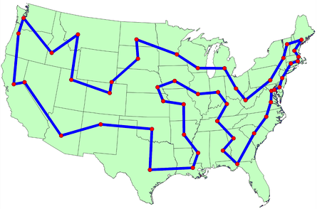
TSP Example
Given a list of cities and the distances or costs between each pair of cities, the goal of the Traveling Salesman Problem (TSP) is to find the shortest possible route that visits each city exactly once and returns to the starting city. This is an NP-hard problem!
Brute Force: Try all possible permutations of the cities and find the one with the minimum cost. \(\Theta((n-1)!)\)
Dynamic programming: Use a table to store the minimum cost of visiting a subset of cities.
Branch and bound: Use a tree to store the partial solutions and prune the branches that cannot lead to a better solution.
Greedy algorithms: Start with an empty tour and add the next closest city to the tour.
Metaheuristic algorithms: Genetic algorithms, simulated annealing, etc.
Paradigms To Be Covered
Brute Force
Exhaustive Search on all possible solutions.
No heuristic, no pruning, no optimization.
Only feasible for small problem instances.
Exact algorithms.
Solves enumeration problems thus can also solve searching, optimization, decision and counting problems.
Examples: Combinations, Permutations, TSP, knapsack, etc.
Backtracking
Try out possibilities until a solution is found or all possibilities are exhausted.
Backtrack to the previous decision point if a partial solution cannot lead to a solution.
Examples: N-queens, Sudoku, graph coloring, etc.
Greedy
Make the locally optimal choice at each step.
Usually leads to a suboptimal solution.
Examples: Prim’s algorithm, Kruskal’s algorithm, Dijkstra’s algorithm, Huffman coding, etc.
Paradigms To Be Covered (cont’d)
Divide and Conquer
Divide the problem into smaller subproblems.
Solve the subproblems recursively.
Solves independent subproblems or ignore the dependency and overlapping factors.
Combine the solutions to the subproblems to obtain the solution to the original problem.
Examples: Merge sort, quick sort, binary search, etc.
Dynamic Programming
Divide the problem into smaller overlapping subproblems.
Systematically solve the subproblems and store the solutions in a table.
Top-down (recursive with memoization) or bottom-up (iterative).
Examples: Fibonacci numbers, knapsack, TSP, etc.
Other Groups To Be Covered
Self-balancing tree related
AVL tree
B-tree
Graph related
Minimum spanning tree
Shortest path
Randomized Algorithms
Introduce randomness into the algorithm.
Pseudo-random number generator and seed.
Examples: Genetic Algorithm, Randomized quick sort, Monte Carlo algorithms, Las Vegas algorithms, etc.